
Internet searches for polar alignment of a telescope mount using the drift method yields many hits. The tutorials I have seen talk about measuring drift of star trails for stars in two directions, one near the equator at the meridian, the other east or west near the horizon. Two directions are needed because each is only sensitive to the mount's polar misalignment in one direction. The need for two stars and an iterative procedure that goes back and forth between them it is said makes the method cumbersome and time consuming. For these reasons this method is not very attractive (I haven't actually used the method).
As you know, a camera sitting on a tracking, perfectly aligned mount is stationary with respect to the stars and will see no tracks, neglecting refraction. With the polar axis pointed away from the pole by some angular distance, the camera sees tracks in proportion to that misalignment. Conceptually it important to understand that the tracks arise from the fact that the camera is rotating with respect to stars, and that this rotation has an axis determined by the mount's polar-axis misalignment. The crucial point is to recognize that that axis of rotation is perpendicular to the Earth's north pole, i.e., an axis through the equator somewhere – where depending on in what direction the mount's axis is miss-pointed. When the camera is pointing towards or near that axis of rotation, it cannot see trails. It is like a camera fixed to the Earth pointing at the pole. Thus the need for two camera orientations when using the drift method of alignment: each cannot see trails for misalignments causing rotations whose axis is on the camera's line of sight.
What is missed by the authors of these drift-alignment tutorials is that there is one camera orientation that can see trails regardless of the polar-axis misalignment — this being the pole, simply because the axis of rotation is always on the equator where the camera's line of sight is not. Furthermore, the direction of the star trails at and around the pole reflects the orientation on the equator of the axis of rotation caused by the misalignment. In a way this is counterintuitive because the poles are where we see the stars not move or move very slowly. But what a camera sees on a tracking mount is very different, and exposures of the pole alone are sufficient to perform polar alignment by the this drift method.
Below I've provided three proofs that this drift method for polar alignment works. The first is empirical, where I've photographed drift in a polar field when the polar axis of the tracking mount is intentionally pointed high, low, east, and west of the celestial pole. The photos clearly show drift orthogonal to the direction the mount's axis is pointed relative to the celestial pole. The second is a numerical simulation that takes into account the earth's rotation, the mount's axis pointing relative to the pole, and the tracking mount's counter rotation. The simulation employs rotation matrices, and the graphical results also clearly show the expected drift direction for different polar-axis pointings. The third is an algebraic calculation in the Lie algebra of the rotations, which maps the fixed celestial sphere to a rotating one fixed to the Earth, to the perspective of the polar axis of a mount fixed to the earth and slightly misaligned, and finally to the camera's perspective counter rotating about the mount's polar axis.
The goal of this test is to measure the dependence of the direction of star trails in the viscinity of the pole while tracking, on the pointing of the polar axis. The possibilities are that there is none; that it depends on where in relation to the pole the star is located as well as the pointing of the polar axis; or that the trails are the same everywhere in the field of view, regardless of the location of the pole, but depending of the pointing of the polar axis. It is only the last case that is useful for polar alignment, the only one that gives a definite direction of star trails as a function of pointing alone, and one where star-trail pointing can be used to infer polar-axis pointing.
The equipment is a Canon 350D, a Canon 75-300 mm zoom lens with the lens set at 300 mm, and an Orion Atlas mount. The left-right field of view of the camera and lens is 4.2 degrees. When pointing at the pole, the camera was oriented on top of the mount so that it was approximately upright, i.e., left in each image is west, right is east, and up and down are toward and away from the zenith, respectively. I first took four pictures, each about three minutes of exposure time with the polar axis pointed a few degrees above, below, left, and right of the pole. To determine the direction of drift while tracking, the aperture was covered for 30 seconds starting 30 seconds into each exposure. The idea of blocking the aperture to show the direction of trailing of the stars came from the internet somewhere, and worked well in these exposures.
Below is shown the full field of view, at one-third scale when expanded, of the image taken with the polar axis pointed a few degrees left of the pole. This is the only photo of the four showing Polaris. The north pole is a bit off the right edge. All of these photos are shown with inverted colors (printing dark photos empties ink cartridges). They also are of raw pixels showing evidence of the Bayer matrix.
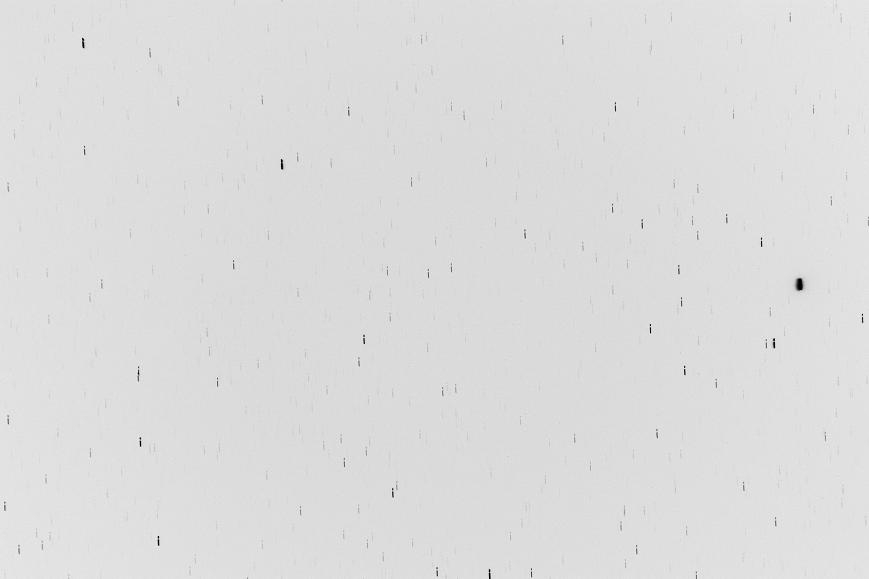
The photo above clearly shows a downward drift of the stars. The crucial thing to note about that drift is that it is uniform over the field of view, and that it does not depend discernibly on angular distance to the north pole. All four of the photos show this uniform drift over the field of view.
Crops of the four photos of polar fields at the full pixel scale to show more clearly the trails are below. Each is oriented with up being up, like with the photo above. The arrangement of the four photos parallels the side of the pole the mount's axis was pointed: approximately above, below, left (west), and right (east) of the pole.
Note the apparent counter-clockwise rotation in the arrangement of photo of the drifts with respect to direction of axis misalignment. From these photos it is evident that the direction of the north pole is an angular distance in a direction about 90 degrees counter clockwise from the direction of the star trails.
We can go further with the data available here. Given that we know the length of the trails in pixels (32 pixels in the photo to the left of the pole), the camera's pixel size, the lens focal length, and the exposure time, we can compute the rate of drift of the stars. This comes to
rate = 32 pixels × 6.4 μm/pixel ÷ 300 mm fl ÷ 3 minutes
= 19 degrees per day
= 1/19 sidereal rate
I'll show in the math section that this drift rate is closely approximated by the product of the sidereal rate and the polar-axis misalignment in radians.
star trails' rate = misalignment (in radians) × sidereal rate
Thus the measured rate tells us the angular distance from the mount's axis to the pole. From data from the first photo, the pole is about three degrees right of the mount's polar axis.
In later sections I'll further show below that the angle between the star trails and the direction from the mount's polar axis to the north pole is closely approximated by 90 degrees, and not just a guess supported by the photos. As you can see, trails provided by a single photo can be very specific about how to reorient the mount's polar axis to align with the Earth's axis. This is the method I suggest using as an alternative to other drift-alignment methods. This is not just theoretical to me; I used polar fields for drift alignment for several years while I was doing astrophotography.
This section provides the results of a numerical test where drift seen by a camera on a tracking mount was computed through rotation matrices. In this calculation a selection of bright stars in a hemisphere containing the north celestial pole are projected onto a plane. Their drifts given two orientation of the mount's polar axis were also plotted on the plane. The selection of stars is shown in the following figure.
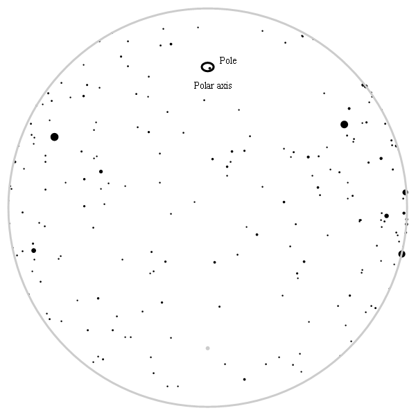
The pole is indicatd by the small oval near the top with Polaris in the interior. Given two orthogonal polar misalignments, drifts are computed and plotted (arrows) in the following two figures. In those figures, the two polar misalignments are shown as red and blue dots, respectively.

And the orthogonal misalignment in the following.

These figures show the drift behavior from the camera's perspective of stars throughout the hemisphere (and particularly near the celestial pole, e.g., Polaris) and that the drift direction is orthogonal to the misalignment of the polar axis. Notice also that there is no drift of the stars along an axis perpendicular to the pole and in the plane of the mount's polar axis with its misalignment, in contrast to the orthogonal direction along the equator where there is drift. This lack of drift in one direction necessitates the use of two camera fields when these fields are on or near the celestial equator. Using the celestial pole as the field obviates that need.
This section is mathematical, and as such it is not for everyone. The methods employed are well known, and I am not claiming anything is original.
The problem is to understand how miss-pointed polar axes generate star trails. This is about rotations, or members of the orthogonal group [2] in three dimensions, SO(3) [3] represented by 3x3 matrices whose transposes are their inverses. The matrix of a rotation about the z axis through an angle $\theta$ looks like this:
\[ R_z(\theta) = \left[ \begin{array}{ccc} \cos(\theta) & -\sin(\theta) & 0 \\ \sin(\theta) & \cos(\theta) & 0 \\ 0 & 0 & 1 \end{array} \right] \]Rotations about the x and y axes are derived from this expression by cyclically permuting the indices. Rotations matrices can be expresses as exponential of their generators. For example, $R_z$ can be expressed as
\[ R_z(\theta) = e^{\theta \sigma_z} \]where $\sigma_z$, called the generator of $R_z $, is the matrix \[ \sigma_z = \left[ \begin{array}{ccc} 0 & -1 & 0 \\ 1 & 0 & 0 \\ 0 & 0 & 0 \end{array} \right] \]
So if the $z$ axis is taken to be the Earth's axis, the Earth's rotation is represented by the matrix $e^{\Omega t \, \sigma_z}$, where the Earth's rotation rate is $\Omega = 2\pi/$sidereal day.
The other two generators, for $x$ and $y$, are
\[ \sigma_x = \left[ \begin{array}{ccc} 0 & 0 & 0 \\ 0 & 0 & -1 \\ 0 & 1 & 0 \end{array} \right] \]and
\[ \sigma_y = \left[ \begin{array}{ccc} 0 & 0 & 1 \\ 0 & 0 & 0 \\ -1 & 0 & 0 \end{array} \right] \]For the purpose of this discussion, the Lie algebra of SO[3] is the vector space spanned by these three generators. These three matrices form a vector of matrices
\[ \vec{\sigma} = [\sigma_x, \sigma_y, \sigma_z] \]from which an arbitrary rotation $R$ can be constructed from three parameters arranged in a vector $\vec{v} = \{a, b, c\}$, \[ R = e^{\vec{v} \cdot \vec{\sigma}} \]
using the inner product $\cdot$. The direction of the vector $\vec{v}$ is the axis of rotation of $R$, and its magnitude is the angle through which $R$ rotates. The exponential of the matrix argument is defined by the power series for the exponential function.
The problem at hand is to compute how the positions of stars as detected by a camera attached to a tracking mount that is misaligned change with time. We had talked about the coordinate transformation from celestial coordinates (relative to the stars) to Earth coordinates (relative to the Earth). Written explicitly, that coordinate transformation can be expressed like this.
\[ \left[ \begin{array}{c} x \\ y \\ z \end{array} \right]_{Earth} = e^{-\Omega t \, \sigma_z} \cdot \left[ \begin{array}{c} x \\ y \\ z \end{array} \right]_{celestial} \] But now the mount axis is offset from the Earth's axis by some angle $\delta$. We can think of that angle as the mount's axis having been rotated away from the Earth's polar ($z$) axis about an axis $\vec{u}$ that passes through the celestial equator. Now we have a rotation that maps Earth coordinates (fixed to the Earth) to coordinates relative to the mount (not tracking yet). \[ \left[ \begin{array}{c} x \\ y \\ z \end{array} \right]_{mount} = e^{\delta \, \vec{u} \cdot \vec{\sigma}} \cdot \left[ \begin{array}{c} x \\ y \\ z \end{array} \right]_{Earth} \]Now we have to talk about the mount's tracking and its matrix. Tracking is there to undo the Earth's rotation leaving the camera stationary with respect to the celestial sphere. In practice there is an error in the pointing of the mount's polar axis, and the mount's counter rotation does not perfectly undo the Earth's rotation. As such, its matrix transforms from the mount coordinates to the camera coordinates like this.
\[ \left[ \begin{array}{c} x \\ y \\ z \end{array} \right]_{camera} = e^{\Omega t \, \sigma_z} \cdot \left[ \begin{array}{c} x \\ y \\ z \end{array} \right]_{mount} \]The map that tells us how the camera sees the stars is the concatenation of these three maps.
\[ \left[ \begin{array}{c} x \\ y \\ z \end{array} \right]_{camera} = e^{-\Omega t \, \sigma_z} \cdot e^{\delta \, \vec{u} \cdot \vec{\sigma}} \cdot e^{\Omega t \, \sigma_z} \cdot \left[ \begin{array}{c} x \\ y \\ z \end{array} \right]_{celestial} \]It is the concatenated exponentials, call it the matrix $M$, that performs this coordinate transformation that we will look at more closely. \[ M = e^{-\Omega t \, \sigma_z} \cdot e^{\delta \, \vec{u} \cdot \vec{\sigma}} \cdot e^{\Omega t \, \sigma_z} \] Notice that if the misalignment angle $\delta$ is zero, then we are left with $M = $ the unit matrix, i.e., perfect tracking.
From here, we are looking for a power series in the time variable $t$, the first-order term of which is gives us the star trailing. There is an interesting identity that does this for us. Let the variable $x$ be an element of the Lie algebra, e.g., $\sigma_z$. Then define the operator $x:$ to be the operator that acts on a matrix $y$ according to \[y \rightarrow x:y = x \cdot y - y \cdot x \] We are going to identify $x$ with $\Omega t \sigma_z$, so that powers of $x:$ are in powers of $t$. The identity is \[ \begin{array} ee^x \cdot y \cdot e^{-x} & = & e^{x:} y \\ & = & y + x:y + \cdots \end{array} \] So $x:y$ is first order in $t$ and is the interesting term.
The exponential in $y = e^{\delta \, \vec{u} \cdot \vec{\sigma}}$ is also expanded to a power series, the terms of which are powers of the misalignment angle $\delta$. \[ y = 1 + \delta \, \vec{u} \cdot \vec{\sigma} + \cdots \] where '1' is the identity matrix. We are interested in the term first order in $\delta$. Using $x = Omega t \sigma_z$, \[M = 1 + \delta \Omega t (\sigma_z \cdot (\vec{u} \cdot \vec{\sigma}) - (\vec{u} \cdot \vec{\sigma}) \cdot \sigma_z) + \cdots \]
Note the identity \[(\vec{a} \cdot \vec{\sigma}) \cdot (\vec{b} \cdot \vec{\sigma}) - (\vec{b} \cdot \vec{\sigma}) \cdot (\vec{a} \cdot \vec{\sigma}) = (\vec{a} \times \vec{b}) \cdot \vec{\sigma} \] where $\times$ is the vector cross product. This identity reflects that the Lie algebra of the space spanned by the generators and the algebra of vector cross products are the same. Using this identity and $\sigma_z = \hat{z} \cdot \vec{\sigma}$, \[ M = 1 + \delta \Omega t (\sigma_z \times \vec{u}) \cdot \vec{\sigma} + \cdots \]
In other words, to first order in time $t$ the camera sees the celestial sphere rotating at rate $\delta \Omega$ about the axis $\sigma_z \times \vec{u}$. That rotation is proportional to $\delta$, and if $\delta$ is zero, there is no rotation – as expected. The axis of rotation is perpendicular to the axis $\vec{u}$ that represents how the polar axis is rotated from the celestial pole (earth's axis), which is on the celestial equator, and also perpendicular to the $z$ (Earth's polar) axis. This means that stars in polar fields always trail. So the rate at which, and in what direction, the stars trail in a polar field are consistent with the evidence from the previous two sections, and quantitatively tell us how to repoint the polar axis.
I further think that this method could be a high-precision alignment method, particulaly among those already with the talent for the two-star drift alignment method. When algorithms are used that quantitatively privide corrections to the mounts polar axis, such as those employed by some go-to mounts and third-party software, convergence may be quite fast. One can also employ longer exposures when making fine adjustments, or even two exposures separated by an hour or more, and use the blink method to sense motion. Then an axis correction can be computed and applied to the mount.
This picture may be overly optimistic, especially in light of the views expressed in reference [1]. But I am sure both the speed and the practically achievable accuracy of polar-axis alignment can be pushed using this method.