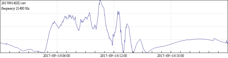
sidmon is a python program for receiving and recording signal intensities in the VLF frequency range using a computer sound card and the alsaaudio package. It can record multiple stations simultaneously. In my tests there is no amplification of the antenna signal or other signal conditioning besides antenna tuning. See the equipment section below for a description of my setup. The first graph is an example of the system's performance, showing a plot of NPM with a small SID.
The program employs a few signal-processing tricks that result in very low noise levels. The most important is that the code accurately estimates the frequency-dependent background level so that it can be removed before line intensities are measured. The second is to detect and exclude from processing transients in the data stream. These features require setup, and the steps outlined in the next section will give a indication of how they process the data stream.
Once transmitter intensities are measured by sidmon they are output to a file with a header more or less like the Stanford SID file headers. More than one transmitter may be recorded to this file.
This software employs alsaaudio, which seems can only be installed on linux platforms. I've run it only on Ubuntu. I'm told that alsaaudio has problems on fedora 23 and Debian on a Beagle Bone Black.
First identify the sound interface using alsaaudio's arecord program. Use alsamixer to set the capture device (mic or line in) and volume-control levels.
arecord -L
alsamixer
Run the program from its directory giving the sound-device name with the -d switch.
./sidmon.py -d plughw:U5 -lp 1 --nodata
A line is printed to the console and a graph (the -lp 1 switch) is updated each cycle. Data will not be recorded because of the --nodata switch. To exit the program enter exit

The peak in the spectrum is there because the antenna is tuned. The spectrum from an untuned antenna is much flatter.
This graph assists in two tasks. The first is identification of suitable transmitters. A zoomed in view:
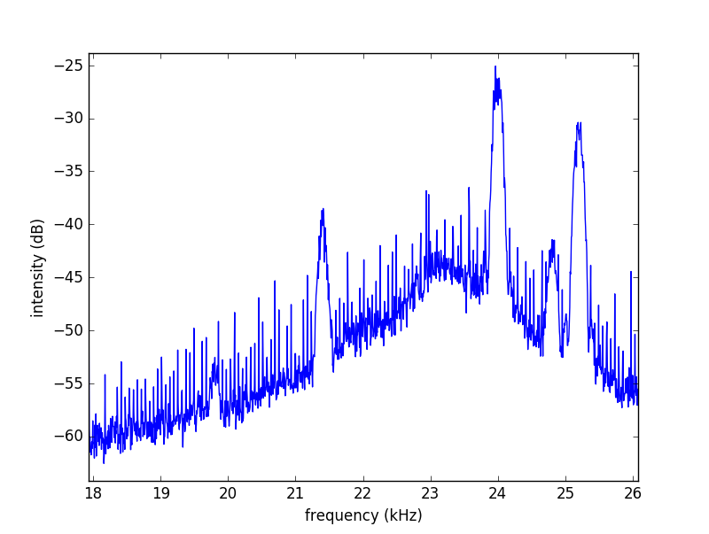
Note also that in spite of the comb of noise lines, the program can extract intensity with good precision.
The ones I monitor are visible in this graph: 19.8 kHz (NWC), 21.4 kHz (NPM), 24.0 kHz (NAA), 24.8 kHz (NLK), and 25.2 kHz (NML). NWC is a weak station, but it nevertheless provides useful intensity. Incidentally, its intensity typically shows seven nulls over sunrise.

Use this link to identify transmitters. Modify the Header.txt template to your circumstances, i.e., name, location, transmitter names and frequencies, etc. Only the # stations and # frequencies lines are essential to the operation of the program.
# stations = NWC, NPM, NAA, NLK, NML
# frequencies = 19800, 21400, 24000, 224800, 25200
A second round of background estimation employs a polynomial fit. The transmitter lines are superimposed on a frequency-dependent noise background. The problem is that this background varies, and we want measured intensities to not be influenced by this background. sidmon does this using a polynomial fit that is designed to not be sensitive to the transmitter (and other) lines. In this way it provides an accurate measurement of the background noise, and above which it measures the line intensities.
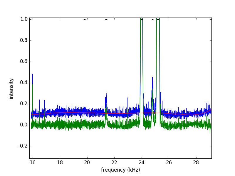
In this plot the blue trace is the first residual spectrum (after the resonance curve has been subtracted as discussed above), the red trace is the polynomial fit to this residual, and the green trace is the second residual. Note that the green trace has an accurate zero baseline. It is from this trace that the line intensities are extracted.
Note that the (red) resonance line of the earlier two plots is actually divided into the raw spectra, meaning that it is a frequency-dependent scaling that makes the spectra approximately flat with respect to frequency. The same resonance line is divided into all spectra, until the program is restarted. The next fit with polynomials differs from spectrum to spectrum, when subtracted moves each spectrum so that its background intensity is accurately set to zero. Measured against this zero background, the line intensities, while not calibrated, are accurately scaled the same from spectrum to spectrum and are accurately proportional to the line intensities. This latter fact is why transmitter intensities show clean nulls over sunrise.
./sidmon.py -d plughw:U5 -l 22900,-17.8,19.5 -v 0.15
The line intensities are saved to a file and a new file is created at the start of each UTC day.
While the program is recording (when run without the -p switch), spectra can be plotted as though using the -p switch by entering a carriage return while the window has the focus. Using this feature, one can check for problems, for instance when the displayed line intensities show a lot of scatter, or to touch up the resonance parameters. A second diagnostic graph is plotted if a character was entered before the carriage return. Note that the program stalls until the plot is closed, so be sure to close it before walking away.
When changing the transmitters being monitored, it is necessary to:
Another noise-reduction feature is the 'veto' feature. I suggest also skipping setup of this feature when first getting your receiver running.
This feature looks for and excludes blocks in the data stream with excess noise. Excess noise can happen when an electrical glitch injects noise into the data stream, which happens when there is lightning in the viscinity. We classify these as transient noise events. Even if they are infrequent, they can still degrade the receiver performance because they are often intense. This is why excluding these noisy blocks can clean up the spectra significantly.
To use this feature, a noise threshold for the exclusion must be set. sidmon is always accumulating a histogram of these block intensities, and when the program is exited after it has been running for a while, this histogram is plotted.
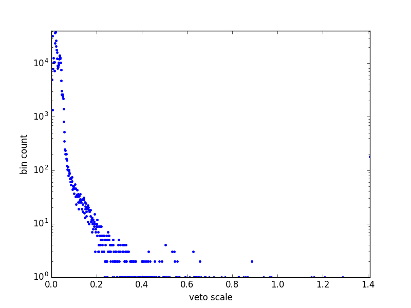
Use this plot to choose a threshold that admits almost all the numerous 'normal' points at lower intensities, but excludes the much-less-frequent higher-value outliers. In the example of the plot above, a choice in the 0.1 to 0.2 range might be suitable. Then rerun sidmon with the-v switch:
./sidmon.py -d plughw:U5 -p -l 22900,-17.8,19.5 -v 0.15
The next question is 'How do I know it is working?'. The lines printed in the command window will give such an indication.

Each line consists of a date and time, followed by the transmitters' line intensities, and finally by a cumulative count of excluded data blocks with excess intensity. If that count stays at zero, then either there are no glitches (maybe), or the threshold is too high. Alternatively, if the count accumulates very rapidly, it is likely that the threshold is too low and should be raised. I would suggest that you set the threshold so that the count accumulates rather slowly and experiment from there.
The final say about this feature's effectiveness is in the number of glitches that are evident in the day's plot of receiver intensities. An example of a glitch is in the first graph in the introduction, at the right edge. There can be many such glitches depending on the severity of the RFI environment, as well as the choice of veto thresholds. Experiment with the threshold from day to day.
The second and optional task is tuning of the antenna. I suggest skipping this step in your first pass at this receiver.
When the antenna is untuned, spectra tend to be flat up to the cutoff of the sound card where the spectra fall off sharply. In the spectrum above, the antenna is tuned and there is a gross peak reflecting this fact near the center of the spectrum. This is due to a 0.06-μF capacitor placed across the antenna terminals, making the antenna resonant at that frequency. When you tune your antenna, a capacitor is wired across the antenna terminal that sets the resonant frequency to the viscinity of the transmitter lines to be monitored. Its value will depend on the inductance of your antenna. With the right value the resonance should look something like in the figures. Use sidmon's ability to generate this plot to help you adjust the capacitor. Tuning benefits sensitivity by filtering out noise at frequencies away from the transmitters you are monitoring.
As was mentioned, sidmon estimates the background noise so that is has a consistent baseline against which to measure line intensities. This ability is key to how quiet and sensitive sidmon is. But a problem that arises is that the resonance due to the antenna tuning is difficult to fit sufficiently well with polynomials. For this reason it is helpful to assist the polynomial fit by providing sidmon with three parameters that roughly fit the resonance. These parameters are the center frequency, the peak intensity, and the quality factor, or Q specifying the width. For my tuned antenna, I enter the -l with three parameters:
./sidmon.py -d plughw:U5 -v 0.12 -l 23250,-27,18.5 -p
which results in graphs that look like this:

The red line in the graphs comes from this switch. It gets subtracted from the blue trace to yield the green trace. The green trace does not have the kink due to the antenna tuning, and is much easier to fit in the viscinity of the kink where the transmitter lines are located.
The three parameters are easy enough to set. The first is set accurately to the center frequency in Hz of the antenna resonance peak in the blue trace. The second is set approximately to the height in decibels of the resonance peak (its value need not be exact). The third parameter, the Q or quality factor of the antenna resonance, takes some iterating. Adjust it to take the kink out of the green trace by stopping and restarting the program with revised values. The result should look something like in the previous graph.
My setup has a loop antenna consisting of 26 turns of 18-gauge wire wound on a one-meter-square spindle. It does this by way of 13 turns of zip cord, spliced to double the number of turns. A length of the cord runs the signal into the house to a 3.5-mm audio plug where there is 0.06 µF across the terminals (obtained by combining three capacitors). Using this capacitance and the resonant frequency (22.9 kHz), the computed antenna inductance is about 80 μH.
I do not use additional amplification between the antenna and the sound card. The gain itself is not needed as there is plenty of signal intensity available. Gain can still benefit sensitivity if it preferentially amplifies the signal over the noise. I also do not use coax to run the signal into the house. Its use is unnecessary.
My sound card is an Asus Xonar U5 with USB interface. It is good for 192 kSps, although I use it at only 96 kSps. I use the line input as opposed to the microphone input because I seem to have enough gain.
The program uses a few percent of the capacity of my four-processor-core computer. The computer runs Ubuntu.
Let me know if you figure out how to install alsaaudio on windows.
Nathan Towne
towne56 at ownmail dot net
10/2017