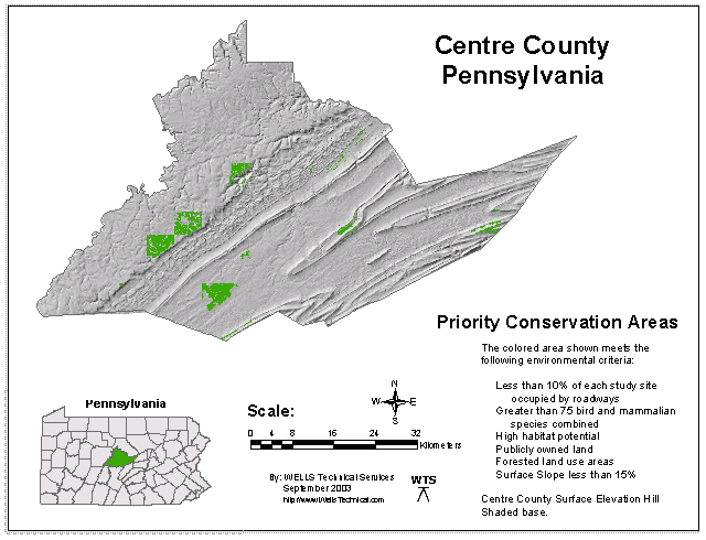
GEOG 5222 Final Project (Lessons 8, 9 & 10) | |
Identifying Priority Conservation Areas in Centre County, Pennsylvania | |
by Tom Wells - September 2003 | |
| Fig.1 - Selected Study Areas |
The final class project required that the students create and implement a work
plan (workflow). The work plan was submitted to the instructor for
approval before the project was completed. This is a relatively complex analysis so multiple approaches are possible
and each student was free to choose their own path. Unlike previous projects,
semi-complete "cook book" instructions were not provided for
possible reference until the
student work plan was approved.
The final project instructions briefly describe the project goal,
the provided data sets, and the environmental criteria used to restrict the
areas of interest. In
brief, we wish to identify priority conservation areas in Centre County,
Pennsylvania that fulfill the following criteria:
My 6 page work plan is available for download as G5222_Final_Project_Plan.doc. The work plan includes comments about the provided data sets and the proposed GIS analysis. The work plan also includes data setup, some pre-processing of the supplied data and some GIS analysis. The proposed work flow was followed to successfully meet the project requirements with one extra detail added. Based on the "class room" discussion, the buffered roadways were subtracted from the areas of interest. The appendix section compares the results of this analysis to the official results based on cell count. |
|
The biggest challenge; calculating the percent of each study site occupied by roadways, was completed while developing the work plan. This was done to gain confidence in my approach. The supplied data contains road type information for the entire county but not the buffer sizes specified in the project instructions. Roads, Highways and Interstates that measure 20 meters, 50 meters and 100 meters, respectively, in buffer radius were specified in an added variable. (Instead of writing a VBA program to populate the added buffer radii field, it was easier to simply select the three road types, one at a time, with select by attribute and assign the appropriate buffer radii via a simple calculate field on just the selected records). There are 8,341 road way polylines in the data set. The ArcView / ArcMap Buffer Wizard tool can be used to turn these lines into 8,341 polygons (using the create buffer "based on a distance from an attribute" option). An option is available in the wizard to specify a dissolve operation on the overlapping polygons after their creation but that takes too long even on a relatively fast modern PC. The number of polygons needed to be reduced before the dissolving operation takes place. The official
(recommended) workflow performs a UNION on the buffered roads and the study
sites that meet the greater than 75 bird and mammalian species
combined criteria. Then the non-roadway polygons are dissolved
together for each study site and subtracted from the study site area to
determine the roadway area. My approach was similar in that I also
restricted the roads of interest to just the 36 out of 155 study areas with
greater than 75 bird and mammalian species.
However I used an INTERSECTION instead of a UNION operation and
dissolved the buffered roads in the 36 study site areas instead of the
non-roadway polygons.
The intersection operation produced 52,421 polygons, but never the less, many
fewer than dealing with every roadway in the county and the runtime was
acceptable (roughly ten minutes with an AMD XP1800 CPU). I understand that
the recommended approach is faster because there are fewer non-road polygons
to dissolve together than roadway polygons. Once the roadway polygons were dissolved together in each study area of a interest, a new field was added to the attribute table to contain the 36 roadway areas. This new field was populated with the corresponding polygon's area for each study site of interest based on the Lesson 2 VBA approach. Once the area of the roads was determined, it can easily be compared to the supplied study site areas. Using a select by Attribute query with the road areas / study site areas < 10 % criteria showed that this cut reduces the number of study sites from 36 to 30. Looking at the dissolved roadway map in Figure 1, the 6 unselected (and therefore eliminated) study areas do appear to have the most roads. | |
|
| |
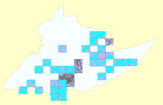
| Figure 1: | Roadways in the 36 Centre County, Pennsylvania study sites with greater than 75 bird and mammalian species combined are shown in Figure 1. Six study sites with UN-highlighted (black) roads have buffered roadway areas that occupy 10% or more of the study site area. Only the 30 study areas with highlighted (turquoise) roads meet both criteria. |
|
At this point the official workflow rasterizes the remaining polygonal based criteria so that they can be considered with the supplied raster based criteria in one final operation. My approach was different in that I combined the polygonal based criteria via the ArcMap GeoProcessing Wizard "Intersect two layers" option first and then only rasterized the final combined results. This worked well because there are relatively few polygons to consider once the roads have been dissolved together. (I.E. computer operations are close to instantaneous.) Figure 2 shows the Habitat Potential in just the 30 study areas that meet the first two criteria. |
|

|
|
| Figure 2: | Centre County, Pennsylvania Habitat Potential in the 30 study sites with greater than 75 bird and mammalian species (combined) and with buffered roadway areas that occupy less than 10% of the study site area. |
|
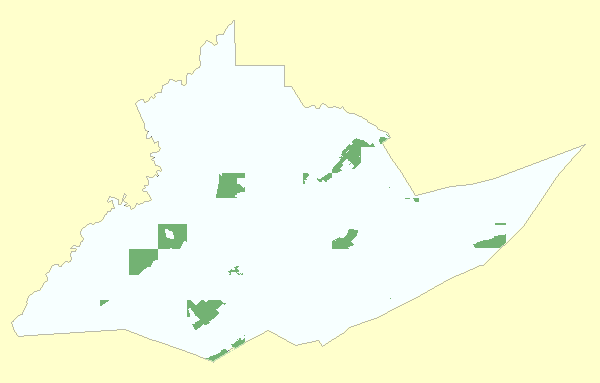
The above figure shows both low and high habitat potential areas. The following Figure 3 shows only polygonal areas that have a high Habitat Potential AND are already Public lands. I.E. Figure 3 shows portions of Centre County that meet the first four criteria listed at the top of this project report. |
|
|
Figure 3: |
The dark green areas shown in Centre County, Pennsylvania meet the first four polygonal based criteria. The 30 study site areas have been reduced to public lands and to areas of high habitat potential. Note: Roadways have not been subtracted yet. |
|
One of the study site areas is shown in detail below in Figure 4 after subtracting the roadways. (The big hole near the center of the site is private property and is easy to spot in Figure 3 above.) It would be hard to see the relatively thin roadways on a small map that covers the whole county so just one study area is shown with some of the surrounding area. Since I had dissolved the applicable roadways together, it was easy to subtract them from the other vector based polygonal shapes via the ArcMap GeoProcessing Wizard "Union two layers" option. (The candidate areas were selected out of the Union results based on zero roadway area in the combined attribute table.) Rasterization has been avoided while generating Figure 4 so the areas of interest are precisely defined. Compare Figure 4 to the rasterized criteria shown in Figure 5 to see the relatively coarse rasterization cell size. |
|
|
Figure 4: |
This particular study site area of interest has relatively few roads, is all high in habitat potential, and all considered rich in species. Only private lands, and roadways subtract from the acceptable (darker) areas. |
|
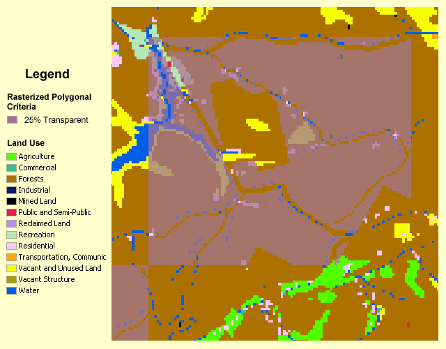
The combined polygonal criteria were rasterized to a 50 meter by 50 meter cell size using the ArcGIS / ArcMap Spatial Analyst "Convert | Features to Raster" option. The cell size was chosen to match the provided land use data grid. Figure 5 shows how the supplied land use data compares to the rasterized polygonal criteria for the same study area shown in Figure 4. The magenta colored rasterized polygonal criteria are shown partially transparent so the land use data is not fully obscured. The combined polygonal criteria were classified into a "1" (Yes) and "0" (no) data value grid. The biggest discrepancy between the two data sets is with regard to "Public and Semi-Public" lands. All of the semi-transparent area is public lands according to the provided polygonal ownership data. However, the land use data includes very little public or semi-public lands. This inconsistency was ignored. Only the forested land use areas were considered in the final analysis. (Forested land is shown as brown areas in Figure 5 and as green areas in Figure 6). Perhaps Public and Semi-Public land use refers to governmental facilities (like libraries, fire houses, etc.) instead of public lands like national and state forests ? |
|
|
Figure 5: |
This figure includes the same study site covered in Figure 4 but with rasterized polygons shown over the Land Use data set. It is interesting to note how the relatively coarse 50 meter by 50 meter cell size roughly approximates the buffered roadways. Some of the roads apparently follow streams as is often the case. |
|
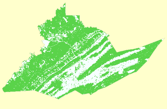
The land use data was reclassified via the Spatial Analyst to produce a data grid with values of "1" (Yes) for forest lands and "0" (no) for all else. The results of the reclassification are shown in Figure 6 and used in the final analysis. The multiple-criteria combination technique was covered in Lesson / Project 7. |
|
|
|
|
|
Figure 6: |
Reclassified Land Use data in Centre County Pennsylvania. The green areas are Forested ("1"). The non-green areas are non-forested ("0") as need for the final analysis calculations. |
|
The last criteria listed at the top of this page is "Surface Slope less than 15%". Surface Elevation data was supplied in a data grid. The Spatial Analyst can easily convert this data grid to a Surface Slope grid via the "Surface Analysis | Slope" operation and thereby make the last criteria a simple reclassification operation. Figure 7 shows surface slope as a percent with the relatively rare steepest slopes (61-180 %) lumped together and colored red. (Otherwise, the four lower classifications are equally spaced at 15 % intervals.) Figure 7 is much prettier than the reclassified yes/no data grid used in the final analysis. |
|
|
|
|
|
Figure 7: |
Centre County Pennsylvania surface slope. The dark green, 0 - 15 per cent, slope criteria was used to restrict the area of interest in the final analysis. |
|
Once all of the criteria have been effectively reduced to a yes/no criteria (with "1" as yes and "0" as no), they can be combined for the final presentation figure (via multiplication). The Spatial Analyst "Raster Calculator" was used to combine three layers into the cells of final interest via the following formula:
Figure 8 shows the final analysis results, areas that meet every
criteria, using ArcMAP's
layout mode. Approximately 26 square miles of Centre County
Pennsylvania meet the specified criteria (as shown in green). The
Centre County surface elevation Hill Shaded base was created using the
Spatial Analysis's default "Surface Analysis | Hillshade"
settings. The Pennsylvania inset map was generated with the provided
Project 5/6 data set. |
|
|
|
|
|
Figure 8: |
Centre County Pennsylvania Priority Conservation Areas according to the listed criteria. A high resolution version of this figure is available in Adobe Acrobat portable document format (pdf) for download as G5222_FP_Fig8-Required.pdf. Note: the downloadable version includes study site boundaries (as white lines). |
|
A fellow GIS student suggested limiting the priority conservation areas to only those that meet some minimum acreage. According to the instructor, ArcMAP is able to perform a "RegionGroup" operation to cluster cells together for such an analysis but that is beyond the scope of this project. The downloadable (pdf) map shows the regularly spaced but somewhat arbitrary Study Site areas. This analysis was simplified to either reject or accept these large study areas. I imagine that a more realistic study would consider bird and mammalian species as a variable and more continuous function in a weighted analysis. It is interesting to note how the town of State College is near, just to the east, of one of the large priority conservation areas identified in this study. I consider State College a very desirable location to live and work in because my wife and I would enjoy camping, hiking and botanizing in the area. |
|
|
Appendix My initial final analysis resulted in 25,948 cells matching all of the specified criteria. This was close enough to the correct multiple choice bonus question to select the correct answer but not as close as expected to the official answer of ~27,000 cells (all 50 meter by 50 meter in size). Did anyone select answer "D. ~1,530 square miles" ? There are "only" 1,118 square miles in the entire county. The immediate suspect was the reclassified surface slope grid because I let the cell size default to the surface elevation grid size of 27.1081 meters on each side. The final analysis results are still based on a 50 by 50 cell size because the other two criteria grids were both based on a 50 meters by 50 meters cell size. (I.E. the final analysis cell size is based on the largest cell size used in the final calculation.) Recalculating the surface slope based on a specified 50 by 50 grid cell increases the final analysis cell count to 26,976 cells because the larger cell size "smoothes-out" the slope and results in less area being restricted by the less than 15 % slope criteria. For example, with the smaller cell size, the maximum slope is 243 % whereas the maximum surface slope with the larger cell size is "only" 173 %. Figure 9 shows how the same study area shown in Figure 4 and Figure 5 is impacted by the surface slope cell size increase in the final analysis. |
|
|
|
|
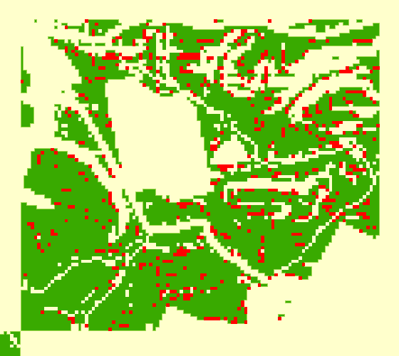
| Figure 9: | The study site of interest with green cells indicating acceptable areas in the final analysis based on either surface slope cell size. The red cells are not included in the final analysis when the surface slope cell size is based on the elevation grid cell size, of 27.1081 meters on each side, instead of 50 meters by 50 meters like the other criteria data grids. |
|
Sources | |
|
|
| Go To the Top of Page | |