GEOG 5223 Project 3 | |
Georeferencing Raster Images | |
by Tom Wells - October 2003 | |
| Fig.1 - Required DRG |
Georeferencing is defined as the process of converting from digitizing
method-imposed coordinates to real-world coordinates. For example, a
digitizing tablet has its own built-in Cartesian coordinate system
independent of the "real" world. Translating coordinates
from a digitizing table to a known coordinate system in the real world
involves georeferencing.
In this lesson, we georeferenced three provided digital files using ArcView 8.3. Two scanned map images and a scanned photograph (from 1963) were georeferenced. Two different transformation methods were utilized to transform the three data sets.
Georeferencing based on just four locations limits the conversion to an "affine" linear transformation. Only three points are required for an affine linear transformation but the use of a fourth point can indicate the degree of transformation accuracy and produce a better compromise fit. Eight intersections (control points) were used to link the photograph to a Road layer shape file. Therefore, a 2nd Order Polynomial could be used to transform (warp) the photo to better fit the roads. |
|
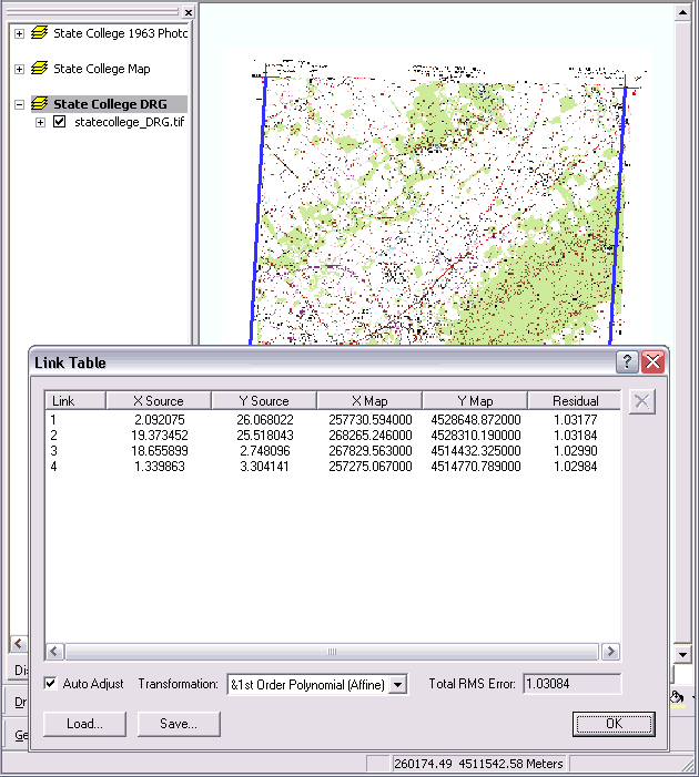
The supplied DRG of the State College 1:24,000 USGS topographic quadrangle was georeferenced using the know coordinates of the four corners. Because it only takes three points (forming a triangle) to define a linear (1st order) transformation, adding a fourth point allows ArcView to make a best linear fit plus calculate a total Root Mean Square (RMS) error. In this case, the Total RMS error is 1.03084 meters (because the map units have been set to meters). The "Rule-of-thumb for georeferencing raster image files is that the RMS Error be less than or equal to one half the map unit size of a cell (pixel)". The standard USGS DRG raster file cell resolution is 250 cells/inch. Since a USGS "topo quad" has a scale of 1:24,000, one inch on the printed map represents 24,000 real world inches or, 250 cells equal 24,000 real world inches. Based on a conversion factor of 0.0254 meters per inch, 1 cell then equals 2.44 meters (on a side). One-half of 2.44 is 1.22 so the Total RMS error reported in Figure 1 is acceptable. | |
|
| |
| Figure 1: | "Lost" DRG file of the State College (PA) USGS Topographic Quadrangle georeferenced in ArcView explicitly based on the four known corner coordinates. - The long blue link lines were generated by reloading the link table AFTER updating the file's Georeferencing data so this DRG file was no longer lost. The Link Table image shown was captured before the update so it shows the georeferencing total RMS error. (The two screen captures were combined using Photoshop 6.0 The blue lines were not avoided because they are instructive.) Note: USGS DRGs are in the UTM, NAD27, coordinate system and State College, PA is in UTM zone 18N. |
|
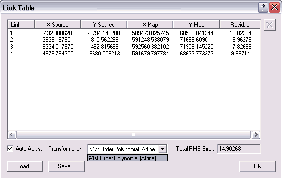
A second raster map imagine was georeferenced using the same temporary transformation link technique employed for georeferencing the Figure 1 map. Four control points with known coordinates were used to explicitly georeference the map. In this case, as shown in Figure 2, the total RMS error is much higher than in the Figure 1 case (even though just the lower right-hand corner of the USGS State College (PA) Topo Quad was scanned). Multiple attempts were made to minimize the RMS error with little impact. The Figure 2 RMS error is approximately seven time larger than the Figure 1 RMS error. The higher error is expected because the georeferenced digital map shown in Figure 1 was derived from a USGS Topo Quad DRG file which is, "for all intents and purposes, distortion-free". The scanned paper image is not of the same quality. According to the lesson # 3 Concept Gallary, a high RMS error results from:.
|
|

|
|
| Figure 2: | Georeferencing the Scanned Image of a Paper Map - The map image file was scanned from the lower right-hand corner of the same State College (PA) USGS Topographic Quadrangle represented by the DRG shown in Figure 1 above. Note: the coordinate system as displayed is "NAD_1927_UTM_Zone_18N", the same as Figure 1. |
|
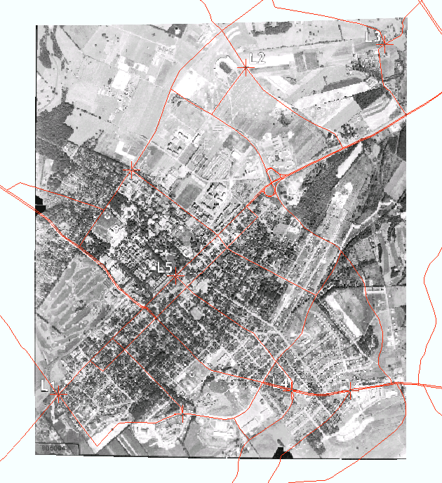
A supplied scanned 1963 photograph of State College (PA) was georeferenced using a graphical technique that links major street intersections to their location on the photo. Then the photo was transformed / warped using a 2nd order polynomial transformation after 8 control point pairs were linked. Figure 3 clearly shows the effect of the transformation because the original photo image was rectangular. An extensive total Root Mean Square (RMS) error discussion (with 5 figures) follows the photographic figure directly below. |
|
|
|
|
|
Figure 3: |
State College (PA) with Major Roads shown in Red. - A photograph was transformed / warped / rubbersheeted in ArcView using selected road intersection as Georeference control points. (Five of the eight control points were specified by the lesson plan and are labeled 'L1' through 'L5' on the photograph.) Note: The shown road layer is in the NAD 1983 StatePlane Pennsylvania North FIPS 3701 projected coordinate system. |
|
The following series of 5 figures shows how the individual "residual" error differences and total RMS error change as linked control point pairs are added or changed. A major change also occurs when the transformation is changed from "1st Order Polynomial (Affine)" to "2nd Order Polynomial". The Residual error was used to spot a probable data inconsistency due to the photo being from 1963 whereas the Road Shape file is much newer. All of the Link Table figures were captured while developing Figure 3. |
|
|
|
|
|
Figure 4: |
1963 State College (PA) Photographic Georeferencing with 3 linked control point pairs. Note how there is no residual error and therefore no total RMS error. This is because it takes all three points (forming a triangle) to define a linear transformation. Hence, there can be no miss-match / residual error. |
|
|
|
|
Figure 5: |
1963 State College (PA) Photographic Georeferencing with 4 linked control point pairs. Note how there is now residual error and hence total RMS error. Only the 1st Order Polynomial transformation is available with 4 points. The large amount of error indicates that the photograph needs to be warped / rubbersheeted via a 2nd Order Polynomial transformation (or higher). |
|
|
|
|
Figure 6: |
1963 State College (PA) Photographic Georeferencing with 6 linked control point pairs. Note how the 2nd Order Polynomial transformation option is now available. With the 2nd order polynomial transformation selected, the residual error becomes very small because every point is used to define the transformation coefficients. |
|
|
|
|
Figure 7: |
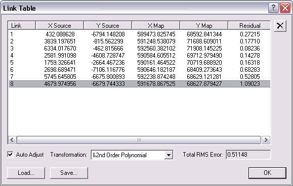
1963 State College (PA) Photographic Georeferencing with 8 linked control point pairs. The error values are no longer small because there are more than the minimum number of link points specified. Therefore a compromise fit is required again.. Link 4 stands out and was modified as explained below to reduce the total RMS error. |
|
|
|
|
Figure 8: |
1963 State College (PA) Photographic Georeferencing with 8 linked control point pairs including one attempted correction. Note how link pair number 4 is now link pair number 8. It still has the highest residual error but the total RMS error has been reduced approximately 75%. Figure 9 shows a close-up of the most problematic intersection. |
|
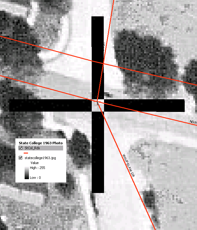
The supplied road layer shape file is considerably newer than the supplied scanned 1963 photograph as indicated by the road layer (StCol_Rds) attribute table. One of the attribute fields is "yr_built" indicating that some roads are as new as 1994 plus a "yr_resurf" field includes years as new as 1999. Apparently much of North Atherton Street is now a two lane boulevard whereas it was a single lane road back in 1963 when the photograph was taken. One of the required link point pairs (L4) is located on North Atherton Street as shown in Figure 9. The photo shows the intersection of two two-way streets whereas the road shape file indicates a typical two-way street crossing a boulevard. I originally linked from L4 to the center of the boulevard crossing. Now L4 is linked to the southern (east-bound) lanes assuming that the original road was reused for that direction. Note: how the extreme zoom shows the residual error of 1.09
meters. |
|
|
|
|
| Figure 9: | Close-Up of North Atherton Street where it intersects Allen Street from the North and Waupelani Drive from the South. Apparently North Atherton Street is now a boulevard according to the StCol_Rds Shape File. Back in 1963 the intersection was very different as shown in the photographic close-up. Note: the entire photograph is shown in Figure 3. |
|
Sources | |
|
|
| Go To the Top of Page | |