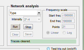
The diagnostics window (_gui2b) of the Matlab control program has a new simple interface to the network analyzer logic (see the screen shot). It mostly implements four scripted measurements described in the primary usage document for the network analyzer: open-loop response, delay measurements, open-loop delay, and proportional gain measurement. There is also a 'manual' measurement mode, and measurements against varying DDS intensity. These options require varying amounts of setup and oversight.
In the network-analyzer box, besides the measurement type selector, there is a selector for the excitation intensity, expressed as a negative power of two in comparison to full scale. The user should be careful with this setting not to over drive the system. Next is a box with controls for the frequency sweep, having a start frequency, end frequency, number of points in the sweep, and a selector for linear versus logarithmic spacing of points. The start frequency should be positive when selecting a logarithmic sweep. Note that this lin/log option is set by the first four options, and so is only available with the 'manual' measurement type. The 'Run' button starts a measurement sequence. The 'Stop' botton does not stop a measurement sequence, but instead switches off the excitation of the system by the DDS.
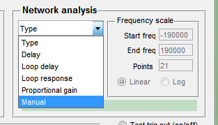
The last option, 'manual', more closely implements the partly-scripted section of the usage document. When using this option, the user sets up the controller and system conditions under which each measurement is made, and then commands the network analyzer to perform a scan. Either linear or logarithmic sweep may be selected by the radio buttons, which are grayed out when the other measurement types are selected..
Every measurement first requires the measurement of a reference response, the first run of each sequence. So no plot will appear after the first measurement of the sequence. Once the reference response is measured, subsequent measurements are compared with this response and plotted on a common mag/phase plot. The phase part of linear-frequency plots will be annotated with the mean delay of the response function.
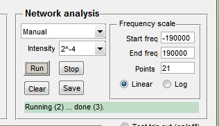
The status line indicates whether a run is in progress or completed. It also shows in parentheses the number of internally accumulated response functions at the start and end of the last run. Measured response functions and other data can be saved to a .mat file using the 'Save' button. The file name is currently fixed at 'naLastMeasurement' in the Matlab working directory. The 'Clear' button reinitializes the network analyzer by clearing the accumulated response functions and the reference response function.
So the manual measurement type resembles the sequence of steps taken when using an analog network analyzer. The system operating point and other conditions are set up as needed. The signal injection point is fixed in the controller at dout40, and pickup points are selected as needed, currently only through the debug multiplexor.
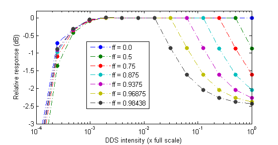
This last measurement type plots response against modulation intensity, where measurements are done at a single frequency. The point is to detect non-linearity, such as clipping or gain compression, in a network. Care must be taken when using this script, however, to avoid over driving the system under test.

The type selection for this measurement is (currently) called 'Gain compression'. Because what is varied is modulation intensity, in contrast to frequency with the other types, the interpretation and use of the controls are different. The frequency at which the measurement is made is selected by the 'Start freq' and 'Relative frequency' controls almost as before. The reference response is measured at that frequency, and at the intensity selected by the intensity control. The intensities at which measurements are all taken are hard coded in powers of two from 20 to 2−10 relative to full scale. Successive runs are plotted together, until the measurement is cleared by the clear button. In the figure, for example, the measurements are taken at frequency 1 kHz relative to IF2, and the reference intensity is at 2−5.
The next figure demonstrates clipping of the signal din1_2, where the DDS signal is mixed with the feed-forward set point. The apparent pattern of the traces is because the ff set point is within successive powers of two of full scale.
It is a simple matter to measure in a bench set up the intensity dependence of the analog electronics (DAC, up conversion, down conversion, etc.) when the controller output is routed to one of the inputs.