Feedback ramp table programming

Overview

The feedback setpoint table is a programmable interpolated waveform generator in logic (RampInterp.v). It provides programmable ramps of the feedback setpoint that are smooth in the sense that the setpoint is changed according to the points of the table, and that the output is linearly interpolated between points. Its intent is for use with the booster rf cavity to program booster ramp cycles, but it can, however, be used in other powered systems utilizing feedback to provide field setpoints. It can provide smooth transitions between setpoints in other systems where one might otherwise program smooth transitions in the host control system.

While the logic can accept arbitrary ramps, given that it interpolates, it is important that ramps as specified by their waypoints be smoothly varying, i.e., free of discontinuities and kinks. Thus to benefit when, in particular, transitioning between setpoints, the controls must retain a memory of the previous setpoint and a smooth 'S' curve be programmed between them. For these reasons the use of the table requires a few steps be performed when the cavity field is changed. These steps are recorded broadly here with more detail following.

1. Given a new field setpoint given in terms of I and Q components, or alternatively magnitude and phase, generate a 512-I/Q pair waypoint table that ramps between the previous setpoint as recorded by the control system and the new setpoint. This should be smooth in the sense of not having kinks, including at the beginning and end.
2. Write the generated ramp to the setpoint table:
   1. Fire the trigger-in end-point (data_write) that resets an address counter addressing the write to the dual-port memory holding the table.
   2. Write the generated waypoint table to the pipe-in end point.
3. Write the inter-waypoint delay, which controls the rate at which the waypoints are clocked into the data stream, to the wire-in end-point rampinterval. The value of this parameter, scaled by 16, is the interval in clocks between output of I/Q-pair waypoints to the data stream. During this interval, each of the interleaved I and Q streams is interpolated.
4. Manually trigger output of the table by firing trigger-in end point ramp_trig. Ordinarily table output is triggered by sources in logic.

Step 1 for generating smooth ramps is discussed in more detail below. In the Matlab interface 'rfboard.m', step 2 is performed by the function fbSPTable.

In step 3, the inter-waypoint delay can have values from 1 to 65535, allowing ramp durations from 0.2 ms to 13.4 s. The ramp duration is

duration = 1/fs × 16 × rampinterval × 512,

where fs is the sample frequency, and rampinterval is the 16-bit unsigned control point. Alternatively,

rampinterval = duration × fs / 8192

In the Matlab interface 'rfboard.m', step 4 is performed by the function ramp_trig.

Computing ramp tables

Before continuing, first a note about the structure of the ramps in the context of the I/Q sampling scheme that shapes the data streams. Sampling of the IF data is every fifth quarter IF cycle, which means that a representation of the I and Q components in the sequence I, Q, -I, -Q, ... at the sample rate is returned by each of the eight ADCs in the revision 8 boards. This sequence structure is also generated by the setpoint table in logic. Memory buffer primitives (RAMB16) in the Xilinx chip are organized into 16384 and 18432 bits (the latter includes parity bits). Thus 1024 sixteen-bit samples, or 512 (I, Q) pairs are accommodated by these buffers.

So the task of writing ramps to these buffers is to compute 512 (I, Q) pairs representing the modulation of the ramp, actually writing the 1024-word block to the table, and then triggering the table to output its interpolated ramp. The table can be triggered repetitively without having to reload the table.

We begin starting at the bottom: generating ramps. There are a couple of low-level Matlab functions available at the moment to help compute ramps. The first, ramp, computes the table from an (anonymous) function. help returns this:

>> help ramp
  Generates an array from a function.  
 
    r = ramp(mag, phase, len, fctn)
 
  Parameters
    mag     is an intensity parameter
    phase   is the phase
    len     is the number of real/imaginary pairs of the table
    fctn    specifies a function representing the functional dependence
            of the ramp
    format  specifies the format of the returned table.
            0  2-d array, each row with index and complex value
            1  2-d array, each row with index, real, and imaginary parts
            2  2-d array, each row with real and imaginary parts
            3  1-d array with real and imaginary parts interleaved
 
  The returned ramp table is the product of the complex magnitude and
  phase, and the function specified by fctn.  fctn may be complex-valued.

One ordinarily uses the last format because it most closely generates the data to be written to the table. So ramp is a fairly general function for computing ramps from analytic and other functions. Note that there is redundance in the mag, phase, and fctn arguments in that fctn can be complex valued. But even so, mag and phase are there for convenience.

A lower-level function is Piecewise, which linearly interpolates the table between a smaller number of specified (x, y) pairs representing waypoints of the ramp. The x values represent an integer index representing a x coordinate, while the y value is a complex-valued number representing the value of the ramp at that index. Thus the length of the array is the difference between the x values of the first and last pairs.

>> help Piecewise
  Piecewise linear arrays interpolated from pts.  
 
    r = Piecewise([x1 y1; x2 y2; ... ], format)
 
  The sequence of x values of pts must be strictly  monotonic.  The y 
  values can be complex.  
 
  format:
    0 - 2-d array with x and complex value in second dim
    1 - 2-d array with x, real, and imaginary parts in second dim
    2 - 2-d array with real and imaginary parts in second dim
    3 - 1-d array with real and imaginary parts interleaved
    4 - 2 multiplied by ++-- ...
    all others - same as 0
 
  The array returned does not include the point at the last x.

So the last waypoint specified is the end point of the ramp, although that point is not part of the returned ramp array. So

Piecewise([0 1; 4 2], 3)

returns the transpose (column vector) of these four I/Q pairs

[1 0   1.25 0  1.5 0   1.75 0]

One usually wants to move the field setpoint between two I/Q values. A more specialized function, SFunction(), does this by generating smooth curves between end points with zero derivatives there.

>> help SFunction
  Generates a smooth table of (I, Q) pairs between start and end points, in 
  a 1-d array.  It uses the inverse sine function between the points.
 
    r = SFunction(start, stop, blksize);
 
  start - the starting (complex) value of the ramp
  stop  - the ending (complex) value of the ramp
  blksize - the number of (I, Q) pairs of the ramp.

So a ramp is generated by, for example,

r = SFunction(2783*exp(1.4i), 12873*exp(1.8i), 512);

which generates an I ramp from 2783*cos(1.4) to 12873*cos(1.8) with length 512, and a Q ramp from 2783*sin(1.4) to 12873*sin(1.8), also of length 512. The result r is a 1024-entry table containing these two ramps interleaved.

Writing and triggering tables

The function fbSPTable() writes an array to the setpoint table,

r = SFunction(1000, 10000, 512);
fbSPTable(ifc, r);

where ifc is the structure representing the rf-board interface returned by the constructor rfboard().

The function rampinterval() is a low-level function used to set the interval in clocks between each I and Q waypoint as output by the ramp.

interval = round(duration/512/16*fs);
rampinterval(ifc, interval, 1);

where duration is in seconds and fs is the sample frequency. With the table loaded, the ramp can be triggered either externally, or via software using the function ramp_trig().

ramp_trig(ifc);

CLS ramp sequence

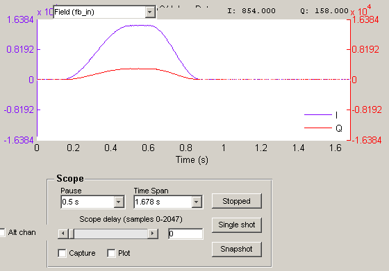
Closed ramp cycles can also be generated using the tools described by concatenating segments. For the closed CLS ramp cycle I concatenated four ramp segments: constant ones for the front porch and extraction energy, and the ramps up and ramp down using SFunction.

z = [ ...
    ramp(abs(injection), angle(injection), interval1, @(x) 1, 3); ...
    SFunction(injection, extraction, interval2); ...
    ramp(abs(extraction), angle(extraction), interval3, @(x) 1, 3); ...
    SFunction(extraction, injection, interval4) ...
];
fbSPTable(ifc, z);

With that, the ramp is waiting to be triggered. SFunction ensures that the segments mate smoothly. The intervals of each segment came from Song's or Jonathan's email. The ramp lasted less than the one-second cycle so that the table was idle and could be retriggered when the next trigger came along. The interval parameter was chosen to match the total duration of the four segments given in the email.

Alternatively, one could have more simply used Piecewise in place of ramp.

All together, generating and loading the CLS ramp looks like this:

z = [ ...
    Piecewise([0 injection; interval1 injection], 3); ...
    SFunction(injection, extraction, interval2); ...
    Piecewise([0 extraction; interval3 extraction], 3); ...
    SFunction(extraction, injection, interval4) ...
];
fbSPTable(ifc, z);

duration = 0.94;
fs = 4e7;
interval = round(duration/512/16*fs);
rampinterval(ifc, interval, 1);

ready for a trigger. This was encapsulated for the purpose into the function CLSRamp,

CLSRamp(injmag*exp(injph*1i), extrmag*exp(extrph*1i), 0.94, 10);

for 0.94-s duration. It is true that the form of the injection and extraction arguments I chose is a bit clumsy.

So a lot can be done using just ramp, Piecewise, and SFunction to generate ramps, although any tools for generating smooth ramps will work.