| Introduction Usage Maps in mixed form Text syntax of optical specifications Ross null corrector examples |
Relating to interior surfaces Drifts, reflection, and refraction Requirements References |
This note is about a library for optical calculations using truncated power series. In contrast to widely-used optical tracking that follows individual rays through optical systems, once-computed optical maps provide a way to succinctly characterize what any starting ray would do in the system. They do this as polynomial functions of the variables at the object surface. Once calculated, these maps can provide optical path-length (wavefront phase advance, actually) maps, which are used to characterize wavefronts and interference, provide first and higher-order optical parameters of the system, and be ray traced. Software implementing truncated power series algebra (TPSA) provide the underlying computational machinery.
With optical path lengths one can compute path-length differences between two optical systems, such as in an interferometric measurement of a mirror and a reference surface. Thus interferometric measurements can be directly compared to models as a means to guide the figuring of optical surfaces. Optical path lengths are calculated using the so-called mixed form where half the independent variables of the map are of the object surface, and half are of the image surface. The mixed form assures that both interference and shearing (where paths taken by the beams differ) are calculated correctly. A surface of interest in the interior of the principal optic may be selected to provide its variable instead of the object surface's variable as an argument of the map and path-length function. This way path length does not have to be mapped back to that surface from another surface as a separate computational step.
Maps may be computed in either two (x, x′) or four dimensions (x, y, x′, y′). Two dimensions allow faster evaluations at higher orders. Non-axi-symmetric surfaces may in general be used; a surface need only preserve the origin. But only symmetric surfaces can currently be implemented in a text specification.
A simple text-based-language specification of optical systems is parsed and evaluated by this library.
The code and examples in this document are written in Visual Basic.Net. Because of the .Net framework, the code should work in conjunction with code in other .Net languages either by attaching the source to a project containing code in other languages, or by calling functions in the dynamic link library Optics.dll. My experience with these options is limited, however.
To be clear, the term path length is used here to mean integrated index of refraction along a path. As such, it times the free-space wave vector is the wavefront phase advance through the path.
An Optics object represents an optical system, describing how rays are carried through the system, and path lengths along the rays. It has five instance variables.
Public m As TPSAMaps
Public pathlen As TPSA
Public rays()() As Double
Public wf4()() As Double
Public wf2()() As Double
The first two are the core optical description of an optic. The variable m contains the map describing how rays are mapped from the starting surface to the ending surface. The variable pathlen is the path length along the paths described by the map m.
The last three are used for plotting. The variable rays contains the points on the ending surface to which m maps a grid of points on the starting surface. This can include points for several angles off axis and several colors. The last two are used for plotting wavefronts, wf2 for two dimensions, and wf4 for four dimensions. These are functions of the final surface instead of the intial (more about this under the method MixedForm).
There are a number of shared members of the class, most of which are initialized when the class is initialized.
Public Shared v, o, n As Integer
Public Shared zero, one As TPSA
Public Shared x, y, xp, yp As TPSA
Public Shared obj, image As Element
Public Shared distortion()() As Integer
The first three are the number of variables, the order, and the number of polynomial terms of the TPSA. The variables zero and one are the zero and unit elements of the TPSA. The symbols x, y, xp, and yp are the TPSA representation of the four variables of optical calculations: x and y for cartesian transverse surface coordinates, and x′ and y′ for the corresponding slopes. When the number of variables is set to two, y and y′ are not initialized. These four shared members are the same as the members of TPSA of the same names. The variables obj and img are predefined for convenience as elements with flat surfaces (see Element class). Finally, distortion is for internal use for removing third-order distortion terms from a map. Access these members by prepending the class name to the variable name, e.g.,
Optics.x
Like with TPSAMaps, Optics is initialized to the number of variables and order with the init method, given as arguments the number of variables and the order as integers to be passed on to the underlying TPSA.
Optics.init(v, o)
The class should always be initialized before any instances are created or referenced.
A new map can be created a number of ways.
Dim x as Optics = New Optics(TPSAMaps.Create.Instantiate)
Dim x as Optics = New Optics(TPSAMaps.Create.PointerOnly)
Dim x as Optics = New Optics(a, b, c, d)          ' specify components (4-d)
Dim x as Optics = New Optics(a, b, c, d, pathlen) ' specify components (4-d)
Dim x as Optics = New Optics(tpsamap, pathlen)    ' using TPSAMaps object

Dim x as Optics = Optics..x      ' x points to Optics.x
Dim x as Optics = Optics.x.clone ' x points to copy of Optics.x

Dim x as Optics
Optics.x.copy(x)	' copies Optics.x to the new variable x
The first instantiates an object with all zero coefficients, while the second creates the pointers m and pathlen (and rays, wf4, and wf2) only. That is, these pointers are set to null. The second and third examples create a map with m and pathlen initialized to the components specified (the first four to m, the last to pathlen). The fifth uses a TPSAMap object, with or without a path length argument. The next two illustrate the use of shallow copies and clones, respectively. The last two lines with the copy method are equivalent to the clone method.
Arithmetic operations on Optics objects are not implemented because they make little physical sense.
Optics has a parser for a simple ascii specification of a sequence of optical elements whose map is to be calculated. This is the higher-level interface to Optics that permits calculations of optical systems. The syntax parallels the table structure of optical specifications in OSLO (ref. 6).
The ascii specification allows a sequence of lines, each line of which is an element. An element consists of a surface specification, type of surface action (reflection or refraction), a drift length to the next element, a glass type, and an optional comment. These specifications are usually separated by semicolons, although equal signs and colons may be used interchangably. For example, an element consisting of +1.5-unit spherical reflecting surface, followed by a −2.3-unit drift through bk7 glass looks like this:
1.5; reflect; −2.3, n-bk7; reflection by a convex mirror
Surfaces have axial symmetry and can be given by several parameters, particularly the radius of curvature, conic constant, and sixth and higher-order corrections to the conic. The number of corrections is not limited. These parameters are separated by commas, and all parameters are optional except the radius of curvature. So a parabolic mirror element might look like this.
−1000, −1; reflect; −500; air; drift to the focus
The first element of a sequence of elements is an object element, whose action parameter is not applicable. The last element of a sequence is the image element, whose only applicable parameter is the surface parameter. So the sequence of elements of a cemented lens doublet with spherical surfaces might be
0; n/a; 0; air;             flat aperture
388; refract; 12; n-sf2;    start of first element
−277; refract; 0; n-bk7;    start of second element
−500; refract; 780; air
0; n/a; 0; air;             flat image surface
To give more detail, the parser returns an array of Element types that are evaluated by the shared function Optic to an Optics optical map. So the refractor example, with the specification in the string variable refr, is evaluated with the code:
Dim seq() as Element = Optics.Parse(refr)
dim map as Optics = Optics.Optic(seq)
A second optical system called the reference optic, as opposed to the test optic, can be specified following a line containing the <section> tag.
; test optic is a parabolic mirror
0; n/a; 2000; air; <aperture>
−2000, −1; reflect; −2200; air
0; n/a; 0; air

<section>

; reference optic is a spherical mirror
0; n/a; 2000; air
−2001.231; reflect; −2200; air
0; n/a; 0; air
When this specification is parsed, Optics computes the two maps and returns an Optics optical map in mixed form consisting of a TPSAMaps object (in the m property) of the test optic, and the difference between the two path-length functions in the pathlen property.
Notice that blank lines and lines starting with a semicolon are ignored. Use of the <aperture> tag is discussed after mixed-form maps are discussed.
Parameters often appear in more than one place in a specification, such as to represent a drift length that is passed through a second time following a reflection. It is convenient to replace those multiple occurrances with a symbol that is given a value at one place in the specification. The latter task is done with a line anywhere in the specification with the following syntax:
variable; name; value
So the specification for a mirror with a null lens starting and ending at the radius of curvature might look like this.
variable; drift1; 88.9
variable; drift2; 26.915
variable; lensROC; 64.8

0; n/a; drift1; air
0; refract; 2; n-bk7
lensROC;  refract;  drift2; air
-80;      reflect; -drift2; air
lensROC;  refract; -2; n-bk7
0; refract; -drift1; air
This functionality is implemented using string substitutions where the variable name and value are both trimmed for leading and trailing spaces.
Parameter optimizations are possible. The object function is the variance of the path length over the surface of interest. The optimizer is a simple one-dimensional function-minimization function that in each iteration computes the minimum point of a quadratic polynomial fit to successive three points computed from the model. It is a not very smart function that usually requires that the minimum be previously bracketed, usually by varying the parameter manually. Multiple parameters may be optimized; in such optimizations the optimizer functions as by nesting one-dimensional optimizations.
The syntax for the optimization with respect to a parameter is the following:
optimize; varname = startvalue : endvalue; tolerance
The values of startvalue and endvalue should nominally bracket the minimum, although convergence of one-dimensional optimizations often occurs without bracketing. As was mentioned earlier, semicolons, colons, and equal signs may be used interchangably. Their usage above mimics Matlab syntax. The optimizer terminates when values of the variable at successive iterations differ by less than the tolerance. A two-parameter optimization of a Ross null corrector for a hyperbolic mirror looks like this:
variable: lens = 129.21;  roc
variable: cc = -1.3452;   conic constant

optimize: drift1 = 140.5 : 141; 0.000001
optimize: drift2 = 1547.3 : 1548; 0.000001

0; n/a; drift1; air;
0; refract; 4.94; n-bk7
-lens; refract; drift2; air;   <aperture>
-1887, cc; reflect; -drift2; air
-lens; refract; -4.94; n-bk7
0; refract; -drift1; air
0; drift; -100; air
0; n/a; 0; air

<section>

0; n/a; 1887; air
-1887.00; reflect; -1987; air
0; n/a; 0; air
The number of variables is two, order is six, aperture is 203.2, and it is evaluated at 0.633 μm wavelength.
Optics has proven useful for the calculation of differences in path lengths of two beams passing through different optical systems. This is the basis of interferometry, where light intensity on a screen is sensitive to the relative phases of interfering wavefronts, and the phases of the wavefronts depend, in turn, on the path lengths taken through the optical systems. (I am using the term path length to include the effect of index of refraction, so that path length times 2π/λ is the wavefront phase advance through that path.) The immediate problem with ray tracing paths is that the maps are calculated starting from an entrance aperture, and a given ray through two systems may not end up and interfere at the same point on the screen (or image sensor). It is essential that path lengths to a given point on the screen be known for the two optical systems, which is to say that path length needs to be calculated as a function of screen position and not as a function of starting point and direction in the entrance aperture. Yet the way that the two systems are illuminated (plane waves or spherical waves) constrains the light at the entrances. So we want a map mmf where the independent variables are, for example, x′ (= 0 for plane waves) at the entrance, and x2 (at the screen), while x at the entrance and x′ on the screen are dependent variables determined by another map mmf.
(x1, x′2) = mmf(x′1, x2)
A map in this form is said to be in mixed form. Alternatively, instead of the light being plane waves, imagine they emanate from a point as spherical waves. Then the independent variables need to be (x1, x2) where x1 = 0. Then we need a map mmf such that
(x′1, x′2) = mmf(x1, x2)
Fortunately, there is an elegant computational method for the conversion of TPSA maps to mixed form. In Optics the method MixedForm returns the mixed form map, the exact form depending on the independent variables needed. With the mixed form for both optical systems calculated, the path lengths may be compared at the screen.
path difference = pathlength2(x′1=0, x2) − pathlength1(x′1=0, x2)
when the light source is a plane wave on the object surface.
The method MixedForm requires an argument that specifies the starting wavefront: whether it is a wave of constant phase at the entrance surface, or a spherical wave starting from a point on the entrance surface.
mf = map.MixedForm(Optics.MF.Surface)
mf = map.MixedForm(Optics.MF.Point)
Here is an example of the wavefront of a parabolic mirror compared to a sphere. The mirror sphere has two-meter radius and 200 mm diameter (f/5). The spherical reference is smaller (100 mm dia). In this model, there is projection lens for focusing the mirror onto the screen. The mirror model is this:
0; n/a; 2000; air
−2000, −1; reflect; −2070; air;     dut
−37.4; refract; −5; n-bk7;          focusing lens
0; refract; −75; air
0; n/a; 0; air;                     screen
and the reference model is this:
0; n/a; 100; air
−101.235; reflect; −170; air;       smaller reference
−37.4; refract; −5; n-bk7;          focusing lens
0; refract; −75; air
0; n/a; 0; air;                     screen
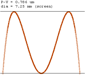
The screen is 150-mm behind the point source. The figure at the right shows the wavefront error across the mirror as it is mapped to the screen. The peak-to-valley error is the marked 0.786 μm.
It is well known that the projection lens is necessary to avoid interference due to edge diffraction. It is also necessary because the P-V (peak minus valley) difference is dependent upon the distance to the screen due to the fact that the two beam take different paths to the screen. That error can lead to over correction or under correction of the mirror while figuring depending on the distance to the screen.
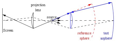
The mirror model below has the 200-mm mirror of the previous example and a Ross null corrector calculated using reference 5 and the null lens of reference 4. A projection lens is shown in the diagram, which is not implemented in these models.
0; n/a; 196.417; air
0; refract; 15; n-bk7
−206; refract; 1573.828; air
−2000, −1; reflect; −1573.828; air
−206; refract; −15; n-bk7
0; refract; −296.417; air
0; n/a; 0; air
The screen is 100 mm behind the point source. The reference model is
0; n/a; 2000; air
−2000.00287; reflect; −2100; air
0; n/a; 0; air

The result is shown to the right, showing very good nulling (note the scale). The wavelength used is 0.633 μm in these examples. In this example, the projection lens is not so necessary because of the quality of the nulling.
With a more aspheric mirror, the nulling is not so good. The next mirror model is:
0; n/a; 135.376; air
0; refract; 8; n-bk7
−129.2; refract; 1085.792; air
−1406, −1.57274, −0.33808, −9.404, −154.16; reflect; −1085.792; air
−129.2; refract; −8; n-bk7
0; refract; −235.376; air
0; n/a; 0; air
and the reference model is:
0; n/a; 1406; air
−1406.0336; reflect; −1506; air
0; n/a; 0; air
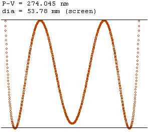
The mirror diameter is 317.5 mm, hyperbolic, with three additional higher-order terms. It is designed for use with a corrector in an f/2 system. The screen is also 100 mm behind the source. The null correction is a factor more than 100 worse than with the 200-mm f/5 mirror, but still a factor of 80 times better than without the null corrector (0.27 μm compared to 22 μm P-V).
The section on mixed form maps showed how to combine beams at the screen for the purpose of computing path length differences to a point on the screen. Notice that the wavefront plots of the previous section are functions of the screen coordinate, and that the screen widths are displayed at the tops of the plots. The distance between the focus and the screen cannot be zero but is otherwise unconstrained, in principle, and the size of the map at the screen depends on that distance and the intervening optics. But the relation between the screen coordinate and the coordinate on the surface of the optical element being tested, in those cases mirrors (call it the test-aperture coordinate), is not specified by the plots or by the mixed-form map, and is in general nonlinear. This means that the screen point scaled to the mirror attributes the path length difference to a point of the mirror different from the actual point from which the path actually came. This is equivalent to shearing, and with an un-nulled significantly aspheric mirror, this can introduce substantial error.
With a projection lens and no other intervening optical elements, the test aperture is imaged through the lens onto the image surface. In that case the only non-linearity of the map between the test aperture and the image surface is due to the distortion of the projection lens itself. If that distortion is small, then the image scaled to the size of the element is equivalent to the mixed-form map of this section. But when the cone angle is large resulting in significant non-linearity of the map due to the projection lens, and/or there are intervening optical elements, such as a null corrector, then non-linearity can still introduce error when figuring aspheres.
Significant or not, a solution of this mapping problem is to compute another mixed-form map, a function of x1 or x′1, and the test-aperture coordinate x2. From here on refer to the test-aperture coordinate with the subscript 2 and the screen coordinates with the subscript 3.
(x1, x3) = mmf 2(x1, x2)
This map is computed from the mixed-form map mmf in a manner similar to the computation of the mmf. The path length function is composed with this map so that it also becomes a function of x1 and test-aperture coordinate x2.
The following example computes the on-axis wavefront of the Hubble Space Telescope design optics with the aperture parameter set to the secondary mirror. The units are millimeters.
; Hubble Space Telescope Ritchey-Chretien optics – as designed
0; n/a; 0; air
−11040, −1.0022985; reflect; −4906.07289; air; <aperture>
−1358, −1.496; reflect; 7406.122; air;		secondary
−1000; n/a; 0; air;				test focal surface
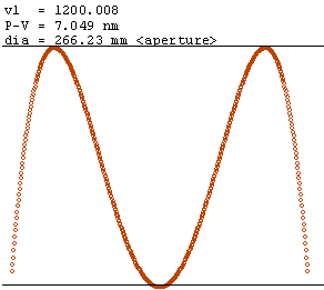
Notice the <aperture> tag showing where the test-aperture variable is to be taken – after the drift of the line to which the tag is attached. In this case it is the secondary mirror. The distance to the screen surface from the focus and the screen's radius of curvature are made the same so that the surface is a constant distance from the focus. The on-axis wavefront is shown in the following plot. Note that the x axis of the plot covers the diameter of the wavefront at the mirror – 266 mm.
The shared function MixedForm (distinct from the method MixedForm) returns the map and path length in an Optics object. If the model is in a string variable hst, then the following code returns the map in the variable htstmap.
Dim hstmap as Optics = Optics.MixedForm(hst, λ, src, dst, dia)
where λ is the wavelength at which the optic is evaluated as a double (immaterial in an all-reflecting telescope), src is the source surface type of the MF enumeration (Optics.MF.Surface in this case), dst is the destination surface type (only Optics.MF.Surface is currently implemented), and dia as a double is the aperture diameter (266 mm).
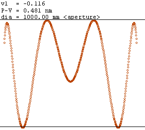
The following optical model comes from a report by J. Burge on testing a 1-m f/3.5 mirror using an Offner null corrector and a point light source. Dimensions come from that report. The plot to the right shows the result. The only parameter changed is a 3 μm final focus adjustment.
; point source 0; n/a; 103.972; air ; null corrector – forward pass 0; refract; 10.386; n-bk7 −41.595; refract; 150.418; air 129.681; refract; 2.924; n-bk7 0; refract; 90.950; air ; drift to mirror 0; drift; 7000; air;; mirror −7000, −1.05; reflect; −7000; air ; null corrector –return pass 0; drift; −90.950; air 0; refract; −2.924; n-bk7 129.681; refract; −150.418; air −41.595; refract; −10.386; n-bk7 0; refract; −103.972; air; drift to focus ; screen 0; drift; −1000.00299; air; focus to screen 1000; n/a; 0; air; spherical screen
Burge mentions nearly perfect correction with a residual error of 0.127 nm rms, which is consistent with the plot.
The core methods of this class library for the construction of optical maps are the shared functions Drift, Reflect, and Refract, which construct the maps for the drift between two surfaces separated in space, reflection by a surface, and refraction by a surface separating two optical media, respectively. These functions are lower-level functions, and as such this section should be considered a topic that can be skipped during a quick read. The drift mathematics is spelled out, but only a short discussion of reflection and refraction is given here.
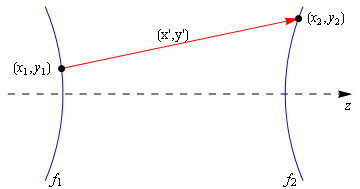
The shared function Drift computes the map (x1,y1,x′,y′) → (x2,y2,x′,y′} between two surfaces as shown in the figure (x and y refer to transverse coordinates).
Drift solves as a power series the equation
x2 = (f2(x2) − f1(x1)) x′ + x1
where the x's are regarded as the (x, y) vectors and the difference f2 − f1 includes the space between the surfaces. This equation is rearranged with separated variables to
x2 − f2(x2) x′ = x1 − f1(x1) x′Now each side is a mapping m of its variable parameterized by x′,
mf2(x2, x′) = mf1(x1, x′)
which has the formal solution
(x2, x′) = mf2−1(mf1(x1, x′)).
The computation of the map mf2−1 is readily implemented using the inverse method of TPSAMaps objects, with the result
drift map = mf2−1 º mf1,where the circle represents map composition. The ease with which this map is computed illustrates the power of TPSA methods as outlined by Berz (ref. 1) and others. Note that the surfaces need be given to an order one fewer than the order of the calculation.
The function Drift takes as arguments the two surfaces as TPSA objects, and the index of refraction of the medium.
Dim f1 as TPSA = −(x^2 + y^2)/(2*R1)
Dim f2 as TPSA = (x^2 + y^2)/(2*R2)
dim d as Optics = Optics.Drift(f2, index, f1)
where R1 and R2 are radii of curvature, index is a real index of refraction, and d is declared an Optics object. The index argument is not used in the internal map calculation, but is needed by the path-length calculation.
The computation of maps for reflection and refraction are straight-forward algorithms based on the analytic geometry of reflection and Snell's law, respectively. The components of three vectors used in these algorithms are TPSA objects. In each case, the x and y components of the maps do not change, that is, the maps do not move the rays, but only change their directions.
The case of reflection in the Reflection method is that the component of the ray vector parallel to the normal to the surface is reversed.
The implementation of Snell's law in the Refraction method is slightly more complicated, but still anchored to the normal of the surface. Glass types are given as a pre-instantiated object of the OptGlass class modeling commercial glass types, plus the object air, which models empty space.
These calculations require, through the normal of the surface, the gradients of the surface with respect to the transverse coordinates x and y. The order of the gradients must be specified to the same order as the calculation.
There are a few other classes of use when using optical maps.