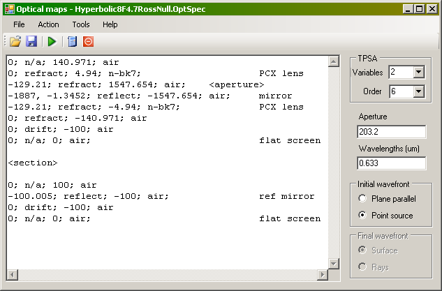
Optical maps is a class for simulating optical systems using truncated power series. This note is about an interface to the Optics class that allows a user to load and save optical specifications, edit them, and plot their wavefronts. In this interface, the number of variables and order of the TPSA, the wavelength of the light, whether the light source is point or parallel, and an aperture may be set. When run, the program sends the specification in the edit window to the optical maps layer for evaluation, after which the resulting map is plotted. More about optical specifications are given elsewhere. A screen shot with a specification for a hyperbolic mirror with Ross-type null corrector, and a spherical reference optic is shown below.
Just to be clear, path lengths are weighted by the index of refraction of the media. So path length times the free-space wave vector is the phase advance through the optic.
Again, a very short list of buttons are available on the tool bar.
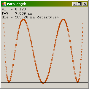
The graph shows the wavefront of the model shown in the screen shot. There are two optical models in the specification, separated by the <section> tag. The first is, in this case, a hyperbolic mirror with a Ross type nulling lens. The second is a spherical mirror. The number of TPSA variables and order are 2 and 6, respectively, the model is evaluated at a wavelength of 0.633 μm, and the span of the plot is 203.2 mm mapped to the location in the first model at the end of the element where the <aperture> tag is located, which is the mirror face. The software plots the difference between the two wavefronts. The two horizontal lines separated by the P-V (peak minus valley) distance 7 nm sets the vertical scale.