GEOG 5222 Project 7 | |
Delineating Ideal Vineyard Acreage in Napa Valley, California | |
by Tom Wells - August 2003 | |
| Land Use Map |
Project 7 introduces the student to Raster GIS Analysis through a relatively complex series of operations that utilize the ArcGIS Spatial Analyst extension. Seven criteria are considered to identify the ideal vineyard acreage in a small portion of Napa Valley, California.
Only acreage that meets every criteria is considered ideal so the analysis is a process of elimination. All of the data is supplied but it must be pre-processed before the process of elimination can be started. Project 7 was described in four parts.
Many operations are new because this lesson / project is the first to utilize the ArcGIS Spatial Analyst. Basically, continuous surfaces composed of 10 by 10 meter cells representing each criteria are created with values of 0 = bad and 1 = good. Therefore these raster surfaces can be multiplied together to produce a surface where a cell value is 1 (good) only where every criteria is met (because zero times any value is zero). A more sophisticated analysis would apply a different weight (level of importance) to each criteria. Many steps are required to complete the required analysis so only selected steps are shown. (This project seemed like more work to me than project 5/6 which covered two weeks instead of one.) The coverage area is approximately 3.3 miles wide. |
|
Figure 1 shows the first Spatial Analyst vector to raster conversion. A "dissolve" was performed on the provided Land Use layer before the raster conversion for training purposes. (Why there are so many polygons in the provided data, is not explained.) The dissolve was unnecessary because turning the polygons into a raster layer eliminates the individual polygon outlines. The raster image is simply a matrix of values (where each value represents a 10 by 10 meter cell, in this case). The hydro line layer and floodplain polygon layer are converted to raster in Lesson 7, Part I too. What attribute field to rasterize on is not specified for the floodplain polygon layer but there are only 3 polygons and # 3 with "TYPE = 0" is the obvious floodplain polygon (that includes the water ways). | |
| Figure 1: | Land Use in a small portion of the Napa Valley, California. This figure was created from a grid of 10 by 10 meter cells. There are 530 rows and 539 columns. |
|
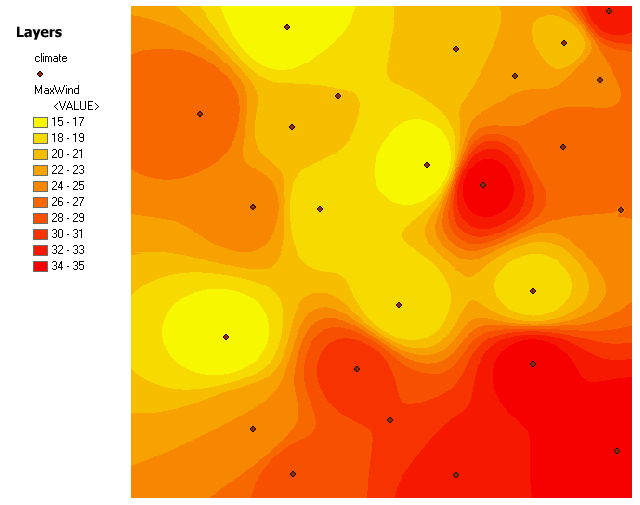
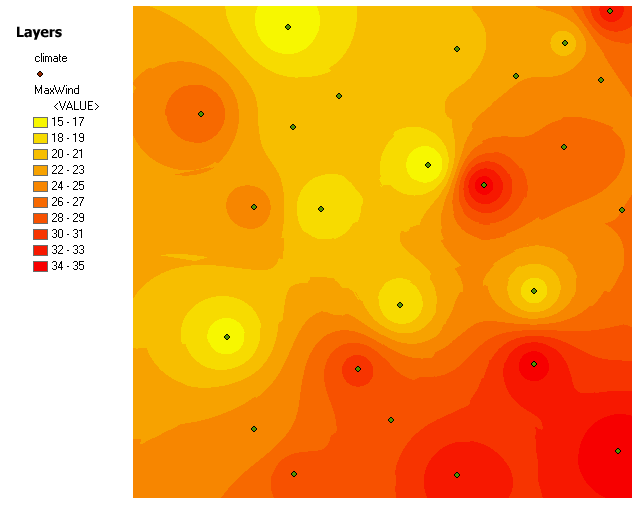
Interpolating Grids from Sample Points Figure 2 and 3 were created in lesson 7 step C of Part II, Performing Surface Operations. Figure 2 shows the "average maximum" interpolated wind speeds used in the vineyard analyst whereas Figure 3 was made for comparison. Both figures use the Inverse Distance Weighted approach to interpolate value grids from discrete locations. Figure 2 uses the required distance weighting factor of 4 whereas Figure 3 shows the default factor of 2 results.
|
|
| Figure 2: | Maximum Wind Speed in a small portion of Napa Valley, California. Supplied climatic data at the points shown were utilized to create a continuous grid / matrix of values. The inverse distance weight factor equals 4 as required for the vineyard analysis. |
|
|
|
|
|
|
|
Figure 3: |
Maximum Wind Speed in a small portion of the Napa Valley, California. Supplied climatic data at the points shown were utilized to create a continuous grid / matrix of values. The inverse distance weight factor equals 2, the default value, for comparison with Figure 2. |
|
Once the supplied data has been rasterized into consistent data grids, a pass-fail data grid (with values of 1 for good & 0 for fail) can be generated via the Spatial Analyst's Reclassify option. This is were the 7 vineyard criteria listed at the beginning of this project page are applied. With only two values, pass-fail grids are not very pretty, but they can be used to mask out acceptable areas and show just the unacceptable criteria (or vice-a-versa). This is demonstrated in Figure 4 where the areas with an acceptable direction of surface slope (aspect) are masked (and colored white in this case) with only the unacceptable values of aspect shown. Slopes facing away from the sun to the north and to the east are considered unacceptable according the vineyard criteria. |
|
|
Figure 4: |
Napa Valley California study area shown with only the unacceptable surface slope (aspect) acreage highlighted. Note: Flat ground is also considered acceptable without any tolerance for a very slight slope. Consequently, limitations in the supplied already rasterized / gridded surface elevation data results in the rejection of some otherwise acceptable areas. |
|
The grids were not combined in the suggested order so that the following figure could be created. Figure 5 shows the suitable sites / acreage in light green with the area removed by the aspect criteria showing in dark green (also see Figure 4.). In general, valleys have relatively smooth surfaces along and near the valley bottom. The supplied already rasterized surface elevation problem appears to have been created from contour lines using a nearest neighbor step-function. Consequently all of the drop occurs along contour lines as appears to be the case on the left / western side of the map. Areas between the contour lines are flat and considered acceptable whereas the areas along the contour line are considered unacceptable because they face north and/or east. In reality, the "contour line areas" are probably just as flat as the adjacent valley bottom lands and therefore just as acceptable for vine production. |
|
|
Figure 5: |
Ideal vineyard acreage in a Napa Valley California study area. Lesson 7 criteria results are shown in light green with the area removed by less than ideal surface elevation slope (aspect) shown in dark green. For location visualization, 50 % transparent elevation shading is shown with underlying light source shading in the less than ideal areas. Note how apparent the "contour line areas" are on the western / left side of the map. |
|
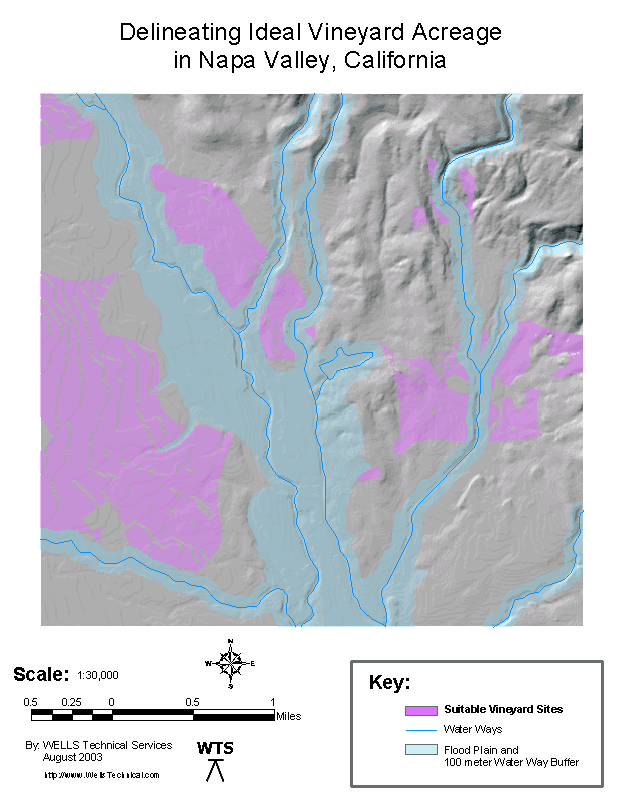
The presentation figure shows the results of all 7 vineyard acreage selection criteria. Layout mode was used to produce a pretty downloadable map. |
|
|
|
|
|
Figure 6: |
Ideal vineyard acreage in the Napa Valley California study area. (A location inset map would be nice...) A high resolution Adobe Acrobat (pdf) file is available for download and printing on "A" size paper (8.5" by 11"). |
|
|
|
|
Optional In general, vineyards can not be located on public lands. The ownership layer data set was downloaded from PSU.edu to add this one additional criteria to the selection process and further restrict the ideal acreage to only private lands. |
|
|
|
|
|
Figure 7: |
Ideal vineyard acreage in the Napa Valley California study area including the optional ownership criteria (in addition to the seven required criteria). This figure is the same as Figure 6 with additional acreage eliminated based on Public ownership. |
|
The ideal acreage for a vineyard in the study area (based on the supplied data and criteria) is on valley bottom land outside of the flood plains. In our area of the country around Lake Michigan, fruit tree orchards and vineyards are located on higher ground to avoid frost damage. Frost is more likely to occur in low lands because cold air sinks into the valleys at night. Vineyards seem more common on the side of hills where as orchards are more commonly found on the top of hills near Lake Michigan. Napa Valley, California has a considerably warmer climate than the area surrounding Lake Michigan so valley frost is apparently not a problem. |
|
|
Sources | |
|
|
| Go To the Top of Page | |